Two Datasets, One Map
By the end of Dive 2 you have produced two completely separate datasets:
-
Acoustic bathymetry. A sparse cloud of (lat, lon, depth) points. Coordinates are absolute, anchored to the float's GPS. Horizontal resolution is roughly 1–2 m at swimming speed; vertical resolution is sub-meter.
-
Photogrammetric mesh. A dense 3D triangulated surface of your target feature. Coordinates are relative — the mesh is internally consistent but has no inherent geotag and no inherent absolute scale. It is essentially a 3D model floating in space.
These two datasets describe the same physical world. Combining them into a single, coherent map is the central technical problem of the course. This module explains how that works.
The Registration Problem
Registration is the process of finding the rotation, translation, and (sometimes) scale factor that aligns one dataset with another. The output is a transformation that, applied to the photogrammetric mesh, places it correctly within the bathymetric coordinate frame.
Three common approaches:
1. Control Points
Place identifiable markers in the survey area before any data collection. Record their GPS positions accurately. Make sure they appear clearly in both the photogrammetric image set and the bathymetric scan. After processing, you tell the software "this corner of the mesh is at this lat/lon/depth" for each marker. The software then computes the rigid transformation that best fits all the markers.
Three markers are the minimum for a rigid transform in 3D space (six degrees of freedom: three translation, three rotation). More markers give redundancy and let you estimate uncertainty.
2. Surface Alignment (ICP)
If your two datasets overlap in space, software can compute the best-fit transformation that minimizes the distance between the two surfaces. The algorithm is called Iterative Closest Point (ICP). It works like this:
-
Start with an approximate alignment (manual or from a partial control point).
-
For each point on the photogrammetric mesh, find the closest point on the bathymetric surface.
-
Compute the rotation and translation that minimizes the sum of squared distances between all these pairs.
-
Apply that transformation. Repeat until improvement falls below a threshold.
ICP works best when there is enough topographic variation that the surfaces can only fit one way. On a featureless flat bottom it fails — the surfaces slide against each other with no preferred alignment.
3. Hybrid
Use one or two control points for a rough anchor, then refine with ICP. This is the most robust approach for recreational sites and is what this course teaches.
Scale
The photogrammetric mesh has no inherent absolute scale. The math of photogrammetry recovers shape and proportion, but not size. To fix the scale, you need a known-distance reference in the image set: a calibrated bar visible in several frames, two control points whose distance you know, or a feature in the bathymetric dataset that you can match to a feature in the mesh.
Without an absolute scale reference, your model is correct in shape but wrong in size by an unknown factor. Always include a scale reference.
Error Budget
Every map you produce must come with a stated accuracy. The typical error budget for this course:
-
Surface GPS on the float: ±3–5 m horizontal. This is consumer-grade WAAS-corrected GPS. RTK GPS would reduce this to centimeters but is out of scope for recreational equipment.
-
Float position uncertainty from tow-line slack and current: ±1–3 m additional.
-
Photogrammetric scale uncertainty (without a reference object): unbounded; with a reference object: ~1–2% of the reference dimension.
-
Combined typical accuracy: ±3–8 m absolute horizontal, sub-meter relative within either dataset.
Your map is not a survey-grade product. It is a recreational documentation of a site, accurate enough for navigation, target identification, and change detection, but not accurate enough for legal boundary or salvage work. Be honest about this when you publish.
Control Points vs Checkpoints
A control point is a known reference used to align the model. A checkpoint is a known reference that you do not use in the alignment; you save it to test how well the alignment worked. For course-level work, use at least three non-collinear control points when practical, and one independent checkpoint when you can. If your checkpoint misses by 4 m, your final map cannot honestly claim 1 m absolute accuracy.
A scale bar is not optional for a scaled photogrammetric model. Without a known distance in the photos, the model may have the right shape but the wrong size. If your scale bar is missing, hidden, moved, or unreadable, say so in the limitations statement.
If you do not have a manufactured scale bar, the pre-measured line from your Surveyor's Pivot kit works as a scale reference too: lay it in frame so it shows up in several shots across the orbit, keeping it off the coral (hold it in the water column or stake it in open sand). Use a low-stretch line or a marked rigid rod, and record the length you actually measured — a stretched cord labeled the wrong length quietly puts that same error into every dimension of your model. And remember the entanglement caution: keep it short, stowed, and managed, never trailing or looped, with your cutter within reach. A rigid rod is the safer choice on both counts.
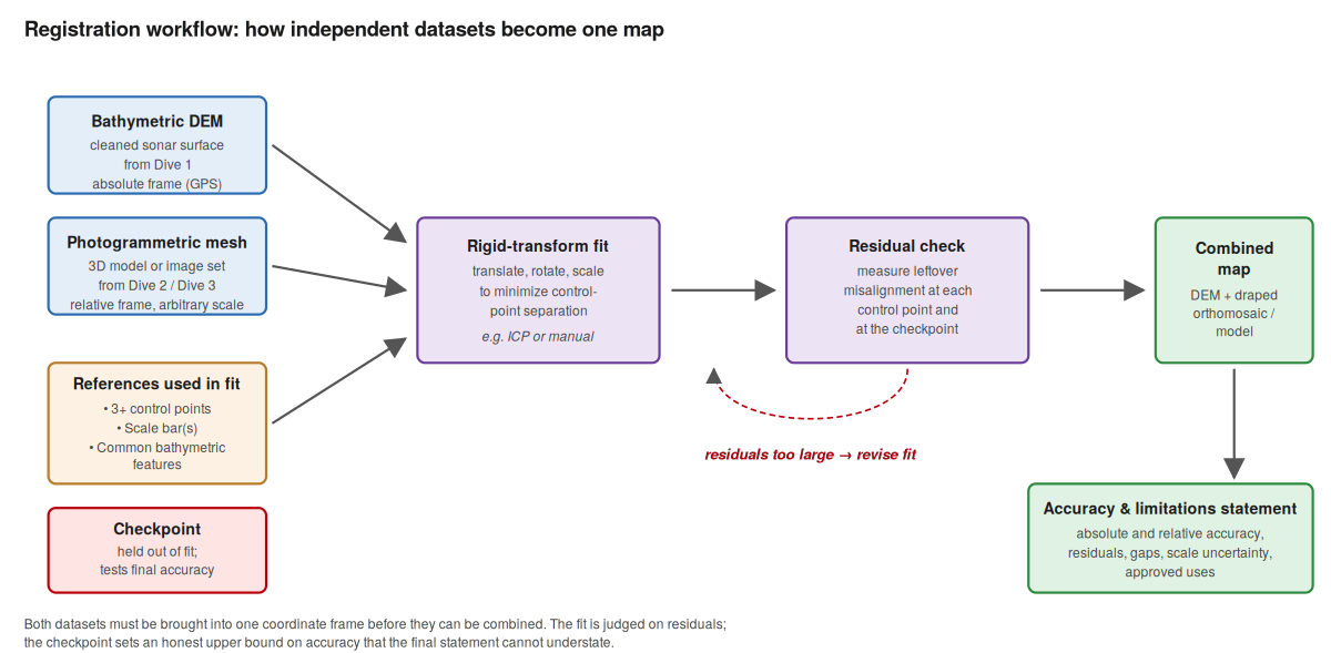
Figure 7. Registration workflow. The bathymetric DEM and photogrammetric mesh are aligned using control points and scale references. Residuals are measured against an independent checkpoint, and the result is published with an accuracy and limitations statement that names the test, not just the hope.
Self-Check
1. Why do you need at least three control points for rigid 3D registration?
2. ICP fails on a flat featureless bottom. Why?
3. Your photogrammetric model is missing a scale reference. The mesh is correct in shape. What do you not know?
Answers
1. A rigid 3D transformation has six degrees of freedom (three translation, three rotation). Each control point provides three constraints (x, y, z position). Two points provide six constraints but the geometry is degenerate — you can rotate freely around the line connecting them. Three non-collinear points fully constrain the transformation.
2. ICP minimizes the distance between matched points on the two surfaces. On a flat surface, any horizontal translation produces zero increase in distance — there is no preferred alignment, so the algorithm cannot converge to a unique answer.
3. You do not know the absolute size. The model could be of an object 1 m across or 10 m across; the proportions are correct but the scale factor is unknown. A known-distance reference fixes this.